Two Software Foundations for Scale

The Gigawatt Machine: NVIDIA, Google, and the Engineering of Scale 4/12

1. Introduction

The B200 and TPU v7 we examined in Article 3 represent the pinnacle of silicon density. But to unlock their trillion-FLOP potential, they require fundamentally different software philosophies: Kernel-Centric (NVIDIA) and Compiler-Centric (Google).

To understand the difference, we must look at the hierarchy of how software talks to hardware.

In any computer, there is a gap between the high-level code a human writes (Python) and the low-level electrical signals a chip understands. There are two competing software foundations to bridge this gap.

The Kernel-Centric Approach (NVIDIA)

In this model, the software controls the hardware step-by-step.

• How it works: The high-level software breaks the AI model down into a sequence of individual operations (e.g., “Multiply Matrix A by Matrix B,” then “Save to Memory”).

• The “Kernel”: For each operation, the system calls a specific, pre-written mini-program called a “Kernel” (from libraries like cuDNN). The GPU executes this kernel, reports back, and waits for the next command.

• The Result: This provides maximum flexibility. Because the software manages every step individually, researchers can easily change the model architecture on the fly without breaking the system.

The Compiler-Centric Approach (Google)

In this model, the software controls the hardware by creating a comprehensive plan upfront.

• How it works: Instead of sending commands one by one, the high-level software sends the entire mathematical graph of the AI model to a Compiler (XLA).

• The Optimization: The compiler analyzes the whole program at once. It looks for efficiencies—like combining three separate math steps into a single hardware action—and generates a single, monolithic binary file.

• The Result: This provides maximum efficiency. By planning the entire route before the data moves, the compiler eliminates the pause between steps, but it makes the system more rigid and harder to change during runtime.

Understanding these two stacks is critical because they dictate how an AI Supercomputer is architected, how models are coded, and how performance is unlocked at the silicon level.

2. The Foundation: CUDA vs. XLA

The deepest point of divergence lies in how the developer interacts with the silicon.

NVIDIA: The CUDA “Kernel” Approach

The foundation of the NVIDIA stack is CUDA (Compute Unified Device Architecture). It allows developers to write “kernels”—C++ functions that execute directly on the GPU’s parallel cores. This model is imperative: the developer (or library author) explicitly manages memory allocation, thread synchronization, and data movement.

• The Mechanism: Most researchers never write raw CUDA. Instead, they leverage libraries like cuDNN (CUDA Deep Neural Network library). These contain hand-written, assembly-optimized kernels for specific operations (e.g., FlashAttention-3 or FP8 Matrix Multiplication). When a framework like PyTorch executes torch.matmul, it dispatches these pre-compiled binaries to the GPU.

• The Trade-off: This requires significant engineering effort to hand-tune kernels for each new GPU architecture (e.g., Hopper vs. Blackwell), but it offers maximum flexibility for dynamic workloads.

Google: The XLA “Compiler” Approach

Google’s TPUs (Tensor Processing Units) leverage XLA (Accelerated Linear Algebra). Unlike CUDA, XLA is not a programming language but a domain-specific compiler. The developer does not write kernel code for a TPU.

• The Mechanism: Frameworks like JAX emit a computational graph. XLA analyzes the entire graph at once. It performs whole-program optimization, fusing multiple operations (e.g., “Add + Multiply + Activation”) into a single hardware instruction to minimize memory access.

• The Trade-off: This approach is deterministic. The compiler calculates the exact clock cycle for every memory movement before the program runs. This eliminates the runtime overhead of managing threads but makes the system rigid; dynamic shapes or conditional branching can trigger costly re-compilations.

Verdict: When is each approach superior?

• CUDA Wins: When Algorithm Velocity is the priority. If you are inventing new layer types daily (e.g., sparse mixture-of-experts, state-space models), CUDA allows you to write a custom kernel and run it immediately without waiting for a compiler to understand the new math.

• XLA Wins: When Production Efficiency is the priority. If your model architecture is stable (e.g., a standard Transformer), XLA can squeeze more performance out of the silicon by fusing operations that a human developer might miss.

Practical Implication for Trillion-Parameter Models

For frontier model training, the “Kernel” approach (NVIDIA) currently dominates because research velocity is paramount. Debugging a compilation error on a 10,000-chip XLA cluster can take days.

However, once a model architecture is frozen, the XLA approach offers a theoretical path to lower training costs by maximizing Model Flops Utilization (MFU).

3. How Close to the Metal is CUDA vs XLA?

To understand the difference between these ecosystems, we must visualize the layers of abstraction between the programmer’s Python code and the silicon transistors.

The NVIDIA Stack (The Layered Hierarchy)

CUDA is not the absolute lowest level of access to an NVIDIA GPU, but it is the lowest level accessible to software developers. It relies on a stack of layers to translate code into action.

• Bare Metal: The physical hardware (Silicon, Transistors, Memory).

• Microcode/Firmware: Internal low-level instructions that control voltage and basic operations. (Inaccessible to humans).

• PTX & SASS: The assembly languages the GPU actually reads. The driver translates CUDA into these machine instructions.

• CUDA: The programming layer. It sits on top of the driver, allowing developers to write C++ code that explicitly manages the GPU’s memory and processor threads.

• Libraries (cuDNN): Collections of pre-written, highly optimized CUDA code for specific math tasks.

• Frameworks (PyTorch): The user-friendly layer that calls the libraries.

The Google Stack (The Direct Compilation)

The XLA approach is flatter. It removes the intermediate “programming layer” (CUDA) entirely.

• Bare Metal: The physical TPU hardware.

• VLIW Machine Code: The TPU requires massive, complex instructions called “Very Long Instruction Words” that control hundreds of chip components simultaneously. This code is too complex for humans to write manually.

• XLA (The Compiler): Instead of a human writing code to manage the chip, the XLA compiler translates the high-level math from the framework directly into the machine code required by the hardware.

The Comparison:

• CUDA is “Close to the Metal” via Control: It allows the developer to manually manage the hardware resources. You explicitly define how to split the work across the chip’s cores and which memory banks to use.

• XLA is “Close to the Metal” via Optimization: It allows the software to generate a monolithic machine-code program that perfectly matches the hardware’s physical layout and timing, without human intervention.

4. Multi-Chip Communication: NCCL vs. ICI

Training large models requires distributing the workload across thousands of chips. The software that orchestrates this data movement differs fundamentally between the two ecosystems.

NVIDIA: NCCL (Hierarchical & Dynamic)

NCCL (NVIDIA Collective Communication Library), pronounced “nickel”, is a topology-aware library designed to navigate the complex, two-tier hierarchy of GPU clusters. It performs runtime discovery of the network topology to route data.

1. Tier 1 (Intra-Node/Rack): Inside a GB200 NVL72 rack, NCCL utilizes NVLink 5.0 to move data at 1.8 TB/s (bidirectional).

2. Tier 2 (Inter-Node): Between racks, NCCL switches protocols to use InfiniBand or Ethernet (RoCEv2) via ConnectX-7/8 NICs.

In-Network Reduction (SHARP): For the Blackwell generation, NCCL leverages SHARP. This offloads collective operations (like AllReduce) to the NVSwitch silicon itself. Instead of GPUs exchanging data and performing summation locally, the switch performs the math as the data passes through it, dramatically reducing latency.

Google: ICI (Flat & Static)

Google TPUs are connected via a proprietary ICI (Inter-Chip Interconnect). Unlike NVIDIA’s hierarchical tree, ICI connects TPUs in a fixed, flat 3D Torus mesh.

• Compiler-Managed Routing: Because the hardware topology is static and known at compile time, XLA manages the communication. There is no dynamic routing protocol or packet headers. The compiler schedules data to move from Chip A to Chip B at specific clock cycles.

• Performance: While ICI often has lower peak bandwidth than NVLink, the elimination of networking overhead results in extremely high utilization for predictable workloads.

When is each approach superior?

• In Cloud/Rental Environments, if you are renting GPUs from Azure or CoreWeave, you may not get a physically contiguous block of racks. NCCL can dynamically detect the topology and route around fragmented allocation.

• If you own the data center (like Google) and can guarantee a perfect 64x64x64 cube of chips, ICI eliminates the massive cost and power overhead of Ethernet/InfiniBand switches.

Practical Implication for Trillion-Parameter Models

The “Flat Mesh” (ICI) is technically superior for 3D Parallelism (splitting a model across Data, Tensor, and Pipeline dimensions) because neighbors are always equidistant.

However, NVIDIA has closed this gap with the NVL72, which effectively creates a “mini-mesh” of 72 GPUs that mimics the TPU’s advantage while retaining the flexibility of NCCL for the broader cluster.

5. NVIDIA’s NCCL Performance from Hopper to Blackwell

NCCL’s performance is directly tied to the hardware it runs on. The advancements from the H100 to the B200 and the new GB200 NVL72 architecture showcase a massive leap in communication speed and efficiency.

DGX H100 (Hopper)

The H100 generation set the baseline for modern AI clusters:

• Intra-Node (within the 8-GPU server): NCCL utilizes 900 GB/s of total bidirectional bandwidth from 4th-generation NVLink.

• Inter-Node (server-to-server): In multi-node scenarios using NDR InfiniBand networking, NCCL sustains communication speeds up to 400 Gb/s across nodes.

DGX B200 (Blackwell “Scale-Out”)

The DGX B200 is the 8-GPU “scale-out” server successor. It doubles the performance on both network tiers:

• Intra-Node: NCCL leverages the 5th-generation NVLink, doubling the total bidirectional bandwidth to 1.8 TB/s (1800 GB/s) within the server.

• Inter-Node: The DGX B200 uses 800 Gb/s networking (via InfiniBand Quantum-X800 or Ethernet Spectrum-X800). NCCL can sustain communication speeds up to 800 Gb/s across nodes, again doubling the previous capability.

GB200 NVL72 (Blackwell “Scale-Up”)

The GB200 NVL72 rack-scale system represents a fundamental architectural shift, and NCCL has been redesigned to exploit it.

• A Single, Massive Fabric: NCCL no longer sees a small 8-GPU node. It sees a massive 72-GPU NVLink domain (which can scale to a 576-GPU pod) where all communication runs on 5th-gen NVLink, providing 1.8 TB/s of bandwidth to every GPU in the entire system.

• In-Network Reduction (INR): This is the most significant performance innovation. The 5th-generation NVSwitch itself has compute engines. NCCL is able to offload the “reduce” (summation) part of the all-reduce operation directly into the network switch. Instead of GPUs waiting to receive data, perform math, and send it on, the switch performs the math as the data is in transit.

This INR feature dramatically accelerates gradient synchronization, freeing up the B200 GPUs’ compute cores to continue working on the next training step, which is a crucial factor in shortening training times for trillion-parameter models.

These hardware advancements, unlocked by NCCL, directly impact the most critical metric: total training time.

Note: Although NCCL is open-source, it is primarily developed and optimized by NVIDIA for their GPUs and networking hardware. Optimal functionality, especially for advanced features like 5th-Gen NVLink, In-Network Reduction, or GPUDirect RDMA, relies on proprietary NVIDIA drivers and libraries.

6. The High-Level Interface: PyTorch vs. JAX vs. TensorFlow

While CUDA and XLA handle the heavy lifting, researchers work in Python. The choice of framework dictates not just the syntax, but how the software interacts with the underlying “Kernel” or “Compiler” philosophy.

PyTorch (The NVIDIA Standard)

PyTorch is the dominant framework for AI research and the training of most large language models (LLMs) today (including GPT-4 and Llama 3).

• Philosophy: “Eager Execution.” PyTorch runs code line-by-line, immediately executing the math on the GPU. This makes it feel like standard Python—easy to debug and flexible.

• The Hardware Connection: It is deeply integrated with the Kernel-Centric (NVIDIA) stack. When you write torch.matmul, it immediately calls a specific pre-compiled CUDA kernel.

• Evolution: To compete with compiler efficiencies, PyTorch 2.0 introduced torch.compile. This captures the model graph and uses TorchInductor to generate optimized kernels, blending its dynamic flexibility with compiler-like speed.

TensorFlow (The Hybrid)

TensorFlow (TF), developed by Google, is the mature incumbent. It sits awkwardly between the two philosophies.

• Philosophy: Originally rigid and graph-based (TF 1.x), it pivoted to “Eager Execution” (TF 2.x) to match PyTorch’s ease of use. It now uses Keras as its high-level API, prioritizing user-friendliness.

• The Hardware Connection: TensorFlow is a hybrid. It works excellently on NVIDIA GPUs (dispatching kernels), but because it is a Google product, it also integrates tightly with XLA. This allows it to run on TPUs, though with more overhead than JAX.

• The Role: While less popular for training new frontier models today, TensorFlow remains massive in production environments due to its robust serving ecosystem (TFLite, TFServing).

JAX (The Compiler Native)

JAX is the modern successor to TensorFlow’s original vision, stripped of the bloat. It is the “purest” expression of the Compiler-Centric philosophy.

• Philosophy: “Function Transformations.” JAX is not a neural network library; it is a math library that supports hardware acceleration. It forces a functional programming style (stateless, pure math).

• The Hardware Connection: JAX is designed specifically to feed the XLA compiler. It uses Just-In-Time (JIT) compilation: it traces your Python function, compiles it into a single binary, and executes it on the TPU (or GPU).

• The Superpower: Because it is pure math, JAX makes parallelization trivial. APIs like pmap (parallel map) allow researchers to split a model across thousands of chips with a single line of code—a task that is notoriously difficult in PyTorch and TensorFlow.

How do they relate?

• PyTorch vs. TensorFlow: These are direct competitors. Both offer a flexible, “Python-first” experience. PyTorch won the research war because its debugging is superior; TensorFlow holds the enterprise ground because of its deployment tools.

• TensorFlow vs. JAX: This is a generational shift. JAX is effectively “TensorFlow done right” for high-performance computing. It discards the baggage of Keras and data loaders to focus entirely on generating the fastest possible XLA graph.

When is each approach superior?

• PyTorch Wins: For Researcher Velocity. If a training run crashes, PyTorch points you to the exact line of Python code that failed. This is invaluable when debugging complex, billion-dollar training runs.

• JAX Wins: For Scaling Elegance. JAX’s pmap (parallel map) and shard_map APIs allow you to describe how to split a model across 10,000 chips in just a few lines of code, whereas PyTorch often requires complex add-ons (like Megatron-LM) to handle distributed training state.

Practical Implication for Trillion-Parameter Models

• Use PyTorch: If you want access to the largest ecosystem of open-source models, tutorials, and engineers. It is the safe, flexible choice for NVIDIA hardware.

• Use JAX: If you are building a custom supercomputer (using TPUs) or if you need absolute maximum mathematical efficiency at extreme scale (50,000+ chips).

• Use TensorFlow: Generally avoided for new frontier model training, but critical if you are integrating into a legacy enterprise pipeline that requires robust mobile or edge deployment.

The industry has largely voted for PyTorch (used by OpenAI, Meta, xAI) simply because the talent pool of engineers who know it is vastly larger.

However, teams that are willing to pay the “JAX Tax” (learning a difficult new language) often report superior stability and efficiency at the extreme scale of 50,000+ chips.

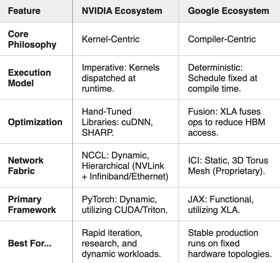
7. Summary: The Engineering Trade-Off

8. Conclusion

Ultimately, the choice between these ecosystems represents a fundamental architectural decision rather than a binary right-or-wrong answer. It is a choice of strategic priority.

The NVIDIA path prioritizes agility. It allows research teams to iterate rapidly, debug easily, and leverage the massive community support of PyTorch. It relies on raw hardware power to mask software inefficiencies, making it the ideal choice for teams exploring the unknown frontiers of model architecture.

The Google path prioritizes efficiency. It demands a more rigorous, structured approach to coding upfront, but rewards engineers with a system that executes with deterministic precision at scale. It transforms the data center into a predictable “math factory,” ideal for stable, massive-scale production workloads.

As we move forward, the lines are blurring—PyTorch is adopting compiler techniques, and XLA is becoming more flexible—but understanding the distinct DNA of these two stacks remains essential for any infrastructure engineer.

In our next article, Article 5, "The Compute Node", we will examine the physical manifestation of the NVIDIA and Google ecosystem: the compute node.